Hai / Bye: syntactic ambiguity in Valence

• Title: Hai / Bye
• Author: Daniel Temkin
• Language: Valence
• Year of development: 2026

Picking up from the main book thread for Forty-Four Esolangs, we'll build a short program in Valence to show how syntactic ambiguity works in the language. It will be the Hai / Bye program, presented in full at the end of this post.

In English, we can form sentences like "Billy saw the group with the telescope," which resolve in two different ways: the group has the telescope, or Billy is looking through the telescope at the group.

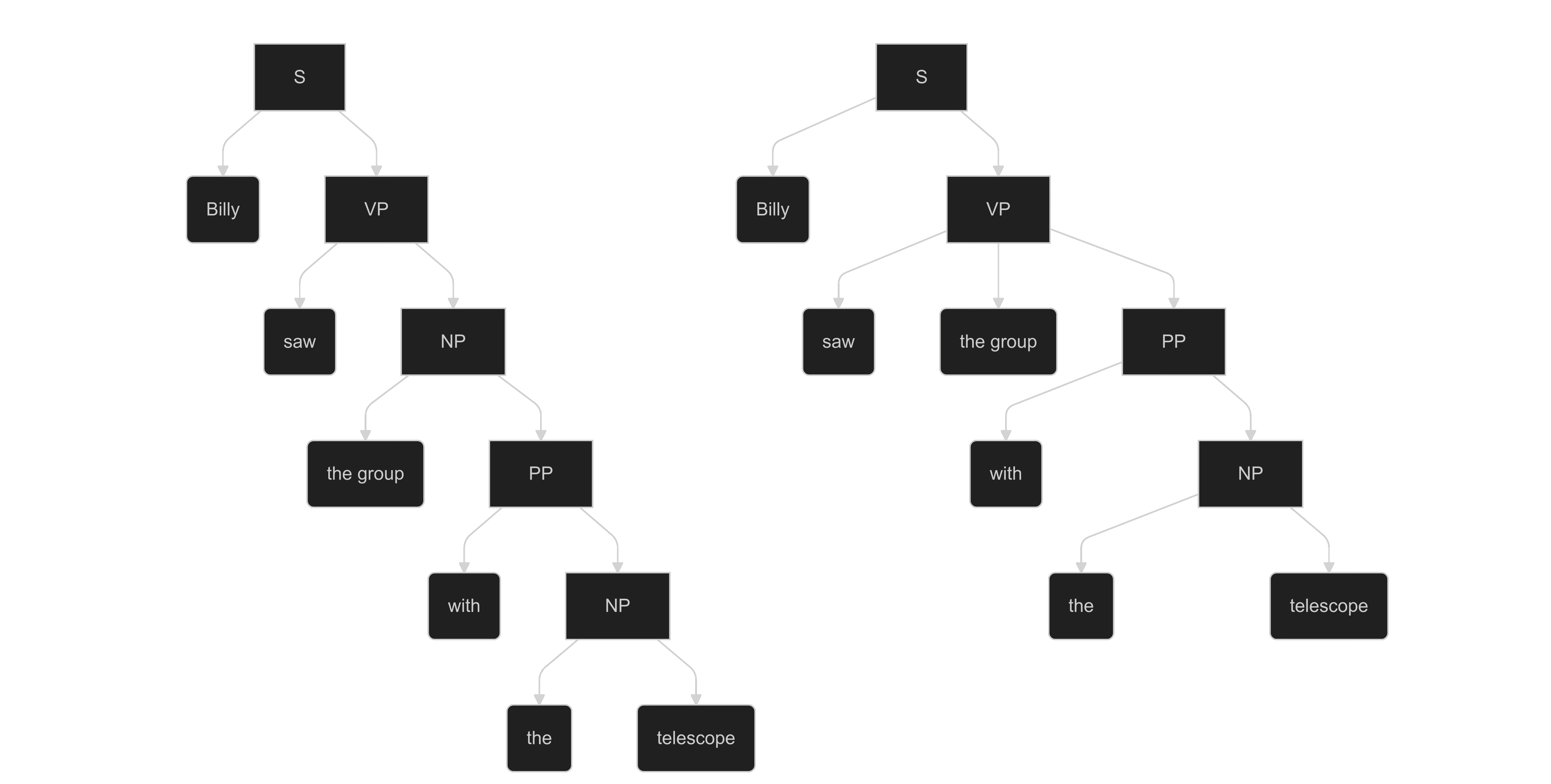
Valence brings to programming this same structural ambiguity, where a line of code can hold multiple interpretations. When running the program, the interpreter forks the program at each ambiguous statement, allowing all versions of the program to play out in parallel. There is no single "correct" reading. This can be tried using the online interpreter / code editor.

Each Valence sign can be a command, an expression, a variable, or a literal value (by default, an octal digit). Its reading is determined by context: whether it is treated as a command vs. an expression, and how many parameters it is given.

Monads (signs that take one parameter), are written prefix. Using 𐅶 as example, it is written 𐅶x for parameter x. When a sign has two parameters, it is written infix,x𐅶y.

Each possible syntax tree for a line of code is evaluated; if we want to lock down these readings, we can explicitly mark a set of signs as a parameter by surrounding them with square brackets.

For example, take the line of code 𐅶𐅶𐅶:

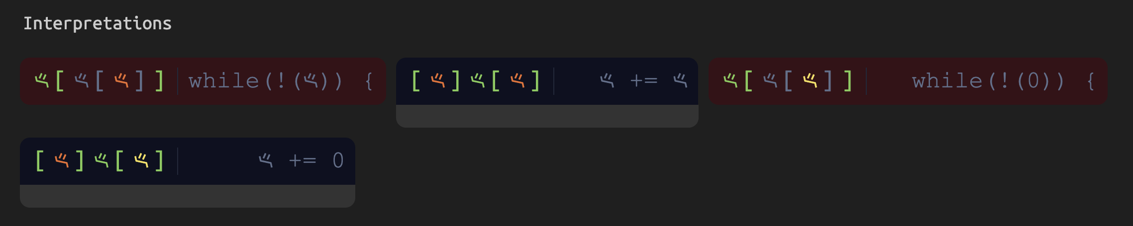
Either the first sign is the command and it's a while loop, 𐅶[𐅶[𐅶]] (these are marked in red as there's a syntax error: the loop is never closed). Or the middle sign is the command, and it's an add/assign (+=), [𐅶]𐅶[𐅶]. The interpreter shows us a version of the code with brackets marking all parameters, with syntax highlighting displaying the command in green.

However, we don't have only two readings but four. There's a second form of ambiguity, because the third sign can be read as either a variable or a literal value (the octal digital zero). We use other signs to explicitly choose one or the other:

𐅶𐅶[𐅾𐅶] locks it down to mean the variable 𐅶, while 𐅶𐅶[𐆇𐅶] indicates the value 0. These are just one use of 𐅾 and 𐆇, which themselves have many different readings.

Here is a longer sample that relies on that second form of ambiguity, between literal vs. variable name:

[𐅶]𐆉𐆇𐆇
[𐆁]𐆉[𐅶]
𐅾[𐆇[[𐅾𐆁]𐅶[𐆇𐅻]]]
[𐆊]𐆉[𐆇𐅶]
𐆉[𐅻]
[𐆉]𐅶[𐆇𐅾]
𐆉[𐆊]
[𐆉]𐅶[𐆇𐅾]

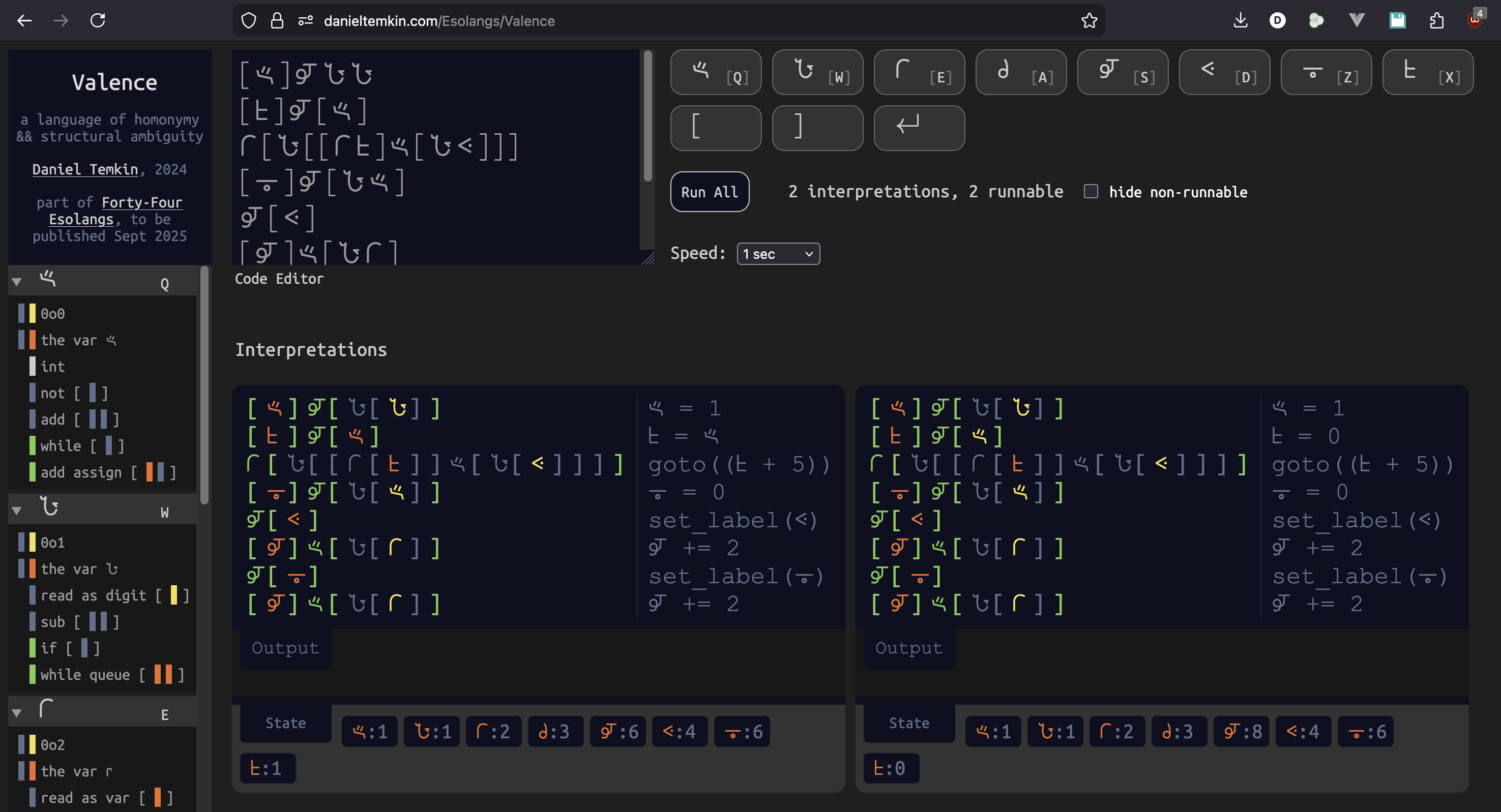
When run in the editor, it has two interpretations, which execute in parallel:

video:

Below each of the two Interpretations are a State box, showing the final state of all Valence variables for that run. There are eight variables in Valence, and each corresponds to one of the signs used in the language. In the first interpretation, 𐆉 ends with the value 6, while in the right, it's given the value 8. Next to each line is psuedo-code showing how the interpreter reads it. For the left version, we have this:

𐅶 = 1
𐆁 = 𐅶
goto((𐆁 + 5))
𐆊 = 0
set_label(𐅻)
𐆉 += 2
set_label(𐆊)
𐆉 += 2

In lines 1 and 2, we assign the value 1 to 𐆁, followed by a goto expression. While Valence allows for structured sequencing with a while loop, it also has goto, which works in terms of labels. On line 5, we set the label 𐅻 (which literally sets the value of 𐅻 to 4 -- not 5, as line numbers are zero-based in Valence). The goto is not to either of those labels, but to the expression (𐆁 + 5). At that point in the program, 𐆁 has the value 1, so this resolves to 6. 6 is an alternate meaning of the symbol 𐆊, so we jump to the label 𐆊.

The right interpretation has a different reading for line 2: 𐆁 = 0. This is because, in the second line ([𐆁]𐆉[𐅶]), 𐅶 is read as both a variable and a literal (the octal value 0o0). As the literal value, we calculate a different label to jump to,𐅻, giving us the value 8 instead of 6. The syntax highlighting helps us read this, as variables are marked in orange and literals in yellow.

NOTE: If an evaluated expression is larger than eight, it mods eight (takes the remainder when divided by 8) to find the label to jump to. If two lines are labeled the same way, it jumps to the closest one

We can build on this to create longer programs that have multiple meanings. Here is the complete Hai/Bye program which extends our existing program, printing either "Hai" or "Bye" to the screen:

[𐅶]𐆉𐆇𐆇
[𐆉]𐆉[𐆇𐆇]
[𐆁]𐆉[𐅶]
𐅾[𐆇[[𐅾𐆁]𐅶[𐆇𐅻]]]
[𐆊]𐆉[𐆇𐅶]
𐆉[𐅻]
[𐆉]𐅶[[𐆇𐅶]𐆇[𐆇𐅾]]
𐆉[𐆊]
[𐆋]𐆉[[𐅻]𐆉[[[𐅻[𐅻[𐆇𐆇]]]𐅶[𐆇𐅻]]𐅶[[𐅾𐆉]𐆁[𐆇𐆋]]]]
[𐅶]𐆉[𐅾𐆋]
[𐆋]𐅶[𐅻[𐆇𐅻]]
[𐆋]𐅶[[𐆇𐅶]𐆇[[[𐅻[𐆇𐆇]]𐅶[𐆇𐆁]]𐆁[𐅾𐆉]]]
[𐅶]𐅻[𐅾𐆋]
[𐆋]𐅶[[𐆇𐅶]𐆇[𐆇𐆊]]
[𐆋]𐅶[[[𐅻[𐆇𐆇]]𐅶[𐆇𐆊]]𐆁[𐅾𐆉]]
[𐅶]𐅻[𐅾𐆋]
𐆋[𐅾𐅶]

Below is the interpretation of that program. The "Hai" and "Bye" differ only in how line 3 is interpreted:

𐅶 = 1
𐆉 = 1
𐆁 = 𐅶 (for Bye) | 𐆁 = 0 (for Hai)
goto((𐆁 + 0o5))
𐆊 = 0
set_label(𐅻)
𐆉 += (0 - 0o2)
set_label(𐆊)
𐆋 = cast(char, (0o105 + (𐆉 * 0o3)))
𐅶 = 𐆋
𐆋 += 0o50
𐆋 += (0 - (0o17 * 𐆉))
𐅶 APPEND 𐆋
𐆋 += (0 - 0o6)
𐆋 += (0o16 * 𐆉)
𐅶 APPEND 𐆋
print(𐅶)

On line 2, we set 𐆉 to 1. In the Bye version of the program, we don't skip line 7, which subtracts 0o2 (octal 2), giving us -0o1. This single change affects all the following calculations.

On line 9, we assign to 𐆋 0o105 + (0o3 * 𐆉), producing 'H' or 'B' depending on the value of 𐆉. This is then copied to 𐅶, which will become our final output string. On lines 11 and 12, we assign𐆋 += (0o50 + (-0o17 * 𐆉)), getting us from 'H' to 'a' or from 'B' to 'y'. For the third character, 𐆋 += -0o6 + (0o16 * 𐆉). Each character is appended to 𐅶, which is printed on the final line of the program.